Plot ranges of data in R
How to control the limits of data values in R plots.
R has multiple graphics engines. Here we will talk about the base graphics and the ggplot2 package.
We’ll create a bit of data to use in the examples:
one2ten <- 1:10
ggplot2 demands that you have a data frame:
ggdat <- data.frame(first=one2ten, second=one2ten)
Seriously exciting data, yes?
Default behavior
The default is — not surprisingly — to create limits so that the data comfortably fit.
Base
Figure 1 shows the default limits. The command to do this is (almost):
plot(one2ten, one2ten)
The actual commands to create this figure and others are below in Appendix R.
Figure 1: Default base graphics plot. 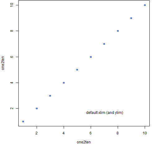
ggplot2
The default here is basically the same, though the resulting picture looks rather different. Figure 2 is created with the commands:
require(ggplot2)
print(qplot(first, second, data=ggdat))
The require command makes sure that the package is loaded into the current R session. In this setting graphs are objects, and they are rendered only when they are printed — hence the call to print.
Figure 2: Default ggplot2 plot. 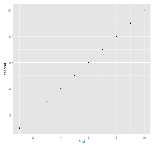
Typical limit
If the default isn’t what you want, you can change it. Here we want — for some reason — more room on the left of the plot.
Base
The simplified version of the command for Figure 3 is:
plot(one2ten, one2ten, xlim=c(-2,10))
Figure 3: Typical use of the xlim graphics parameter. 
The examples here are on the x-axis. To control the y-axis, just substitute “y” for “x” — ylim rather than xlim.
ggplot2
In ggplot2 modifications or additions to a plot object are usually done by adding new terms:
print(qplot(first, second, data=ggdat) + xlim(-2, 10))
Figure 4: Typical ggplot2 specification of x limits. 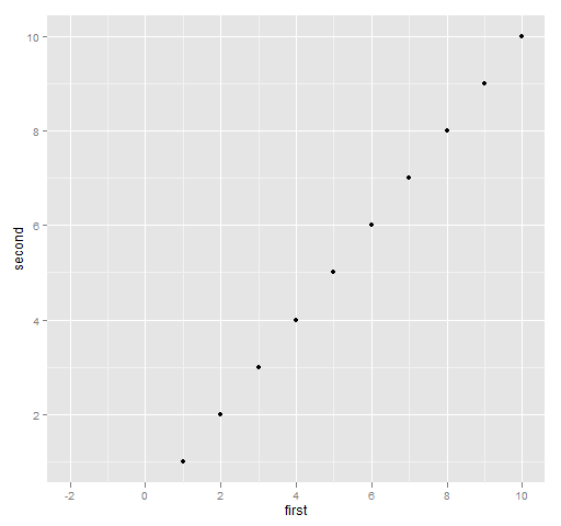
Reverse direction
The first limit need not be the smallest — if not, then the axis is reversed.
Base
Figure 5: Base graph with the x-axis reversed. 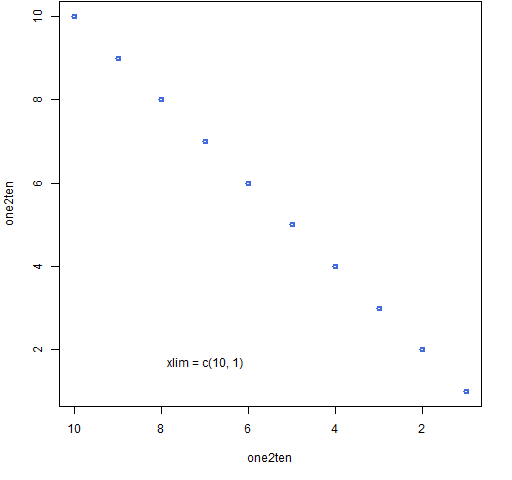
ggplot2
The command for Figure 6 is:
print(qplot(first, second, data=ggdat) + xlim(10, 1))
Figure 6: ggplot2 with the x-axis reversed. 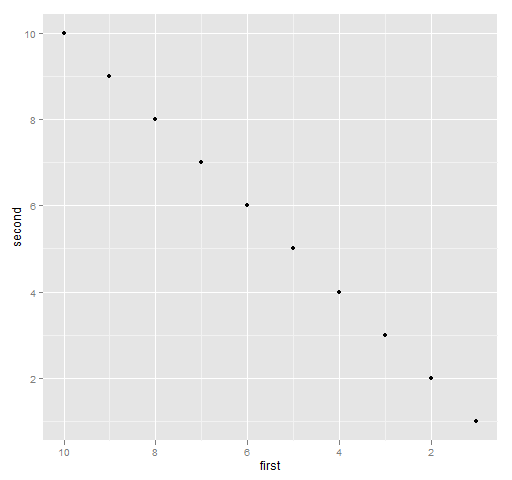
Expansion
The sharp-eyed will have noticed that the actual limits in the plots above are not what is specified. The specifications are strictly inside the plots. This makes it easy to make sure that no data is plotted on the boundary of the plot.
It is possible to change this behavior as well.
Base
We can see what the real range is by looking at the usr graphics parameter:
> plot(one2ten, one2ten, xlim=c(0,10))
> par("usr")
[1] -0.40 10.40  0.64 10.36
You can set some graphics parameters, and some are read-only. The usr parameter can be set, but you almost always want to just use it as is. The first two elements of usr are the x-axis limits, the last two are the y-axis limits.
The x-axis was asked to have limits 10 apart, and we can see that there is an extra 0.4 on each side.
You can force the limits to be taken literally by specifying xaxs (or yaxs for the y-axis):
> plot(one2ten, one2ten, xlim=c(0,10), xaxs="i")
> par("usr")
[1]  0.00 10.00  0.64 10.36
> plot(one2ten, one2ten, xlim=c(0,10), xaxs="i", yaxs="i")
> par("usr")
[1]  0 10  1 10
The "i" stands for “internal”, the other (default) choice is "r" as in “regular”.
ggplot2
Figure 7 is produced with:
print(qplot(first, second, data=ggdat) +
   scale_x_continuous(expand=c(0,0)))
Figure 7: ggplot2 with no x-axis expansion. 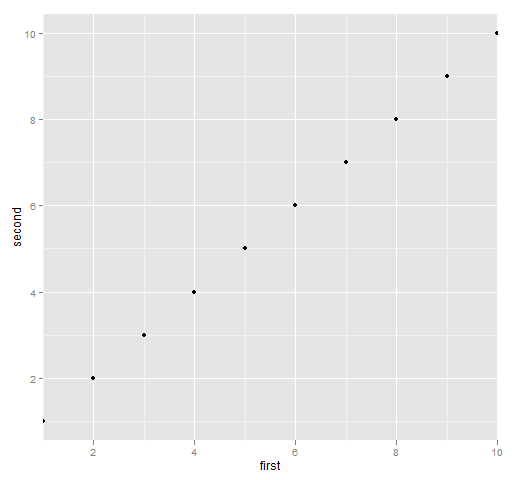
I wasn’t able to both modify the expansion and xlim — I’m not sure if that is a bug or solely due to my ignorance of ggplot2.
Appendix R
The actual commands that created the base graphics are:
Figure 1:
plot(one2ten, one2ten, col="royalblue", lwd=2)
text(7, 1.7, " default xlim (and ylim)")
Figure 3:
plot(one2ten, one2ten, col="royalblue", lwd=2, xlim=c(-2,10))
text(7, 1.7, "xlim = c(-2, 10)")
Figure 5:
plot(one2ten, one2ten, col="royalblue", lwd=2, xlim=c(10,1))
text(7, 1.7, "xlim = c(10, 1)")


Hadley relieved me of some of my ignorance with:
QUOTE
xlim(x) is just a shortcut for scale_x_continuous(limits = x)
so if you want to set both limits and expansion you need
scale_x_continuous(expand=c(0,0), limits = x)
END QUOTE
The following command does as I expect:
print(qplot(first, second, data=ggdat) +
scale_x_continuous(expand=c(0,0), limits=c(-2,10)))
What if you have 2 vectors and you want your plot to automatically scale to the larger instead of the first vector?
Trackbacks & Pingbacks
[…] Plot ranges of data in R (Burns Statistics) […]
Leave a Reply
Want to join the discussion?Feel free to contribute!