The Statistical Bootstrap and Other Resampling Methods
This page has the following sections:
Preliminaries
The Bootstrap
R Software
The Bootstrap More Formally
Permutation Tests
Cross Validation
Simulation
Random Portfolios
Summary
Links
Preliminaries
The purpose of this document is to introduce the statistical bootstrap and related techniques in order to encourage their use in practice. The examples work in R — see Impatient R for an introduction to using R. However, you need not be a user to follow the discussion. On the other hand, R is arguably the best environment in which to perform these techniques.
A dataset of the daily returns of IBM and the S&P 500 index for 2006 is used in the examples. A tab separated file of the data is available at: https://www.burns-stat.com/pages/Tutor/spx_ibm.txt
An R command — that you can do yourself — to create the data as used in the examples is:
spxibm <- as.matrix(read.table(
   "https://www.burns-stat.com/pages/Tutor/spx_ibm.txt",
   header=TRUE, sep='\t', row.names=1))
The above command reads the file from the Burns Statistics website and creates a two column matrix with 251 rows. The first few rows look like:
> head(spxibm)
                    spx        ibm
2006-01-03  1.629695715 -0.1727542
2006-01-04  0.366603354 -0.1359451
2006-01-05  0.001570512  0.6778851
2006-01-06  0.935554103  2.9173527
2006-01-09  0.364963909 -1.4419861
2006-01-10 -0.035661127  0.4106782
The following two commands each extract one column to create a vector.
spxret <- spxibm[, 'spx']
ibmret <- spxibm[,'ibm']
The calculations we talk about are random. If you want to be able to reproduce them exactly, there are two choices: You can save the .Random.seed object in existence just before you start the computation. You can use the set.seed function.
The Bootstrap
The idea: We have just one dataset. When we compute a statistic on the data, we only know that one statistic — we don’t see how variable that statistic is. The bootstrap creates a large number of datasets that we might have seen and computes the statistic on each of these datasets. Thus we get a distribution of the statistic. Key is the strategy to create data that “we might have seen”.
Our example data are log returns (also known as continuously compounded returns). The log return for the year is the sum of the daily log returns. The log return for the year for the S&P is 12.8% (the data are in percent already). We can use the bootstrap to get an idea of the variability of that figure.
There are 251 daily returns in the year. One bootstrap sample is 251 randomly sampled daily returns. The sampling is with replacement, so some of the days will be in the bootstrap sample multiple times and other days will not appear at all. Once we have a bootstrap sample, we perform the calculation of interest on it — in this case the sum of the values. We don’t stop at just one bootstrap sample though, typically hundreds or thousands of bootstrap samples are created.
Below is some simple code to perform this bootstrap with 1000 bootstrap samples.
spx.boot.sum <- numeric(1000) # numeric vector 1000 long
for(i in 1:1000) {
   this.samp <- spxret[ sample(251, 251, replace=TRUE) ]
   spx.boot.sum[i] <- sum(this.samp)
}
The key step of the code above is the call to the sample function. The command says to sample from the integers from 1 to 251, make the sample size 251 and sample with replacement. The effect is that this.samp is a year of daily returns that might have happened (but probably didn’t). In the subsequent line we collect the annual return from each of the hypothetical years. We can then plot the distribution of the bootstrapped annual returns.
plot(density(spx.boot.sum), lwd=3, col="steelblue")
abline(v=sum(spxret), lwd=3, col='gold')

The plot shows the annual return to be quite variable. (Your plot won’t look exactly like this one, but should look very similar.) It could have easily been anything from 0 to 25. The actual annual return is squarely in the middle of the distribution. That doesn’t always happen — there can be substantial bias for some statistics and datasets.
Bootstrapping smooths
More than numbers can be bootstrapped. In the following example we bootstrap a smooth function over time.
spx.varsmu <- array(NA, c(251, 20)) # make 251 by 20 matrix
for(i in 1:20) {
   this.samp <- spxret[ sample(251, 251, replace=TRUE) ]
   spx.varsmu[,i] <- supsmu(1:251,
      (this.samp - mean(this.samp))^2)$y
}
plot(supsmu(1:251, (spxret-mean(spxret))^2), type='l',
   xlab='Days', ylab='Variance')
matlines(1:251, spx.varsmu, lty=2, col='red')
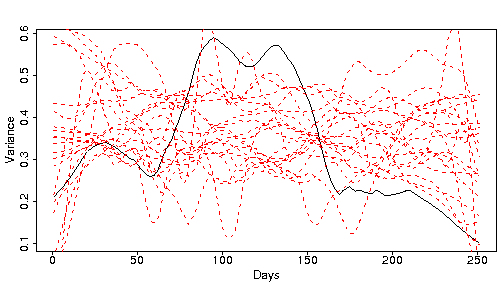
The black line is a smooth of the variance of the real S&P data over the year, while the red lines are smooths from bootstrapped samples. It isn’t absolutely clear that the black line is different from the red lines, but it is. Market data experience the phenomenon of “volatility clustering”. There are periods of low volatility, and periods of high volatility. Since the bootstrapping does not preserve time ordering, the bootstrap samples will not have volatility clustering. We will return to volatility clustering later.
Bootstrap regression coefficients (version 1)
A statistic that can be of interest is the slope of the linear regression of a stock’s returns explained by the returns of the “market”, that is, of an index like the S&P. In finance this number is called the beta of the stock. This is often thought of as a fixed number for each stock. In fact betas change continuously, but we will ignore that complication here.
The command below shows that our data gives an estimate of IBM’s beta of about 0.85.
> coef(lm(ibmret ~ spxret))
(Intercept) spxret
0.02887969 0.84553741
What is after the “>” on the first line is what the user typed (and you can copy and paste), the rest was the response. If we start on the inside of the command, ibmret ~ spxret is a formula that says ibmret is to be explained by spxret. lm stands for linear model. The result of the call to lm is an object representing the linear regression. We then extract the coefficients from that object. To get just the beta, we can subscript for the second element of the coefficients:
> coef(lm(ibmret ~ spxret))[2]
spxret
0.8455374
We are now ready to try bootstrapping beta in order to get a sense of its variability.
beta.obs.boot <- numeric(1000)
for(i in 1:1000) {
   this.ind <- sample(251, 251, replace=TRUE)
   beta.obs.boot[i] <- coef(lm(
      ibmret[this.ind] ~ spxret[this.ind]))[2]
}
plot(density(beta.obs.boot), lwd=3, col="steelblue")
abline(v=coef(lm(ibmret ~ spxret))[2], lwd=3, col='gold')

Each bootstrap takes a sample of the indices of the days in the year, creates the IBM return vector based on those indices, creates the matching return vector for the S&P, and then performs the regression. Basically, a number of hypothetical years are created.
Bootstrap regression coefficients (version 2)
There is another approach to bootstrapping the regression coefficient. The response in a regression is identically equal to the fit of the regression plus the residuals (the regression line plus distance to the line). We can take the viewpoint that only the residuals are random.
Here’s the alternative bootstrapping approach. Sample from the residuals of the regression on the original data, and then create synthetic response data by adding the bootstrapped residuals to the fitted value. The explanatory variables are still the original data.
In our case we will use the original S&P returns because that is our explanatory variable. For each day we will create a new IBM return by adding the fit of the regression for that day to the residual from some day. This second method is performed below.
ibm.lm <- lm(ibmret ~ spxret)
ibm.fit <- fitted(ibm.lm)
ibm.resid <- resid(ibm.lm)
beta.resid.boot <- numeric(1000)
for(i in 1:1000) {
   this.ind <- sample(251, 251, replace=TRUE)
   beta.resid.boot[i] <- coef(lm(
      ibm.fit + ibm.resid[this.ind] ~ spxret))[2]
}
plot(density(beta.resid.boot), lwd=3, col="steelblue")
abline(v=coef(lm(ibmret ~ spxret))[2], lwd=3, col='gold')

In this case the results are equivalent. (An experiment with 50,000 bootstrap samples showed the two bootstrap densities to be almost identical.) There are times, though, when the residual method is forced upon us. If we are modeling volatility clustering, then sampling the observations will not work — that destroys the phenomenon we are trying to study. We need to fit our model of volatility clustering and then sample from the residuals of that model.
R Software
For data exploration the techniques that have just been presented are likely to be sufficient. If you are using R, S-PLUS or a few other languages, then there is no need for any specialized software — you can just write a simple loop. Often it is a good exercise to decide how to bootstrap your data. You are not likely to understand your data unless you know how to mimic its variability with a bootstrap.
If formal inference is sought, then there are some technical tricks, such as bias corrected confidence intervals, that are often desirable. Specialized software does generally make sense in this case.
There are a number of R packages that are either confined to or touch upon bootstrapping or its relatives. These include:
boot: This package incorporates quite a wide variety of bootstrapping tricks.
bootstrap: A package of relatively simple functions for bootstrapping and related techniques.
coin: A package for permutation tests (which are discussed below).
MChtest: This package is for Monte Carlo hypothesis tests, that is, tests using some form of resampling. This includes code for sampling rules where the number of samples taken depend on how certain the result is.
meboot: Provides a method of bootstrapping a time series.
permtest: A package containing a function for permutation tests of microarray data.
scaleboot: This package produces approximately unbiased hypothesis tests via bootstrapping.
simpleboot: A package of a few functions that perform (or present) bootstraps in simple situations, such as one and two samples, and linear regression.
There are a large number of R packages that include bootstrapping. Examples include multtest that has the boot.resample function, and Matching which has a function for a bootstrapped Kolmogorov-Smirnov test (the equality of two probability distributions). The BurStMisc package has some simple functions for permutation tests.
The Bootstrap More Formally
Bootstrapping is an alternative to the traditional statistical technique of assuming a particular probability distribution. For example, it would be reasonably common practice to assume that our return data are normally distributed. This is clearly not the case. However, there is decidedly no consensus on what distribution would be believable. Bootstrapping outflanks this discussion by letting the data speak for itself.
As long as there are more than a few observations the data will reveal their distribution to a reasonable extent. One way of describing bootstrapping is that it is sampling from the empirical distribution of the data.
A sort of a compromise is to do “smoothed bootstrapping”. This produces observations that are close to a specific data observation rather than exactly equal to the data observation. An R statement that performs smoothed bootstrapping on the S&P return vector is:
rnorm(251, mean=sample(spxret, 251, replace=TRUE), sd=.05)
This generates 251 random numbers with a normal distribution where the mean values are a standard bootstrap sample and the standard deviation is small (relative to the spread of the original data). If zero were given for sd, then it would be exactly the standard bootstrap sample.
Some statistics are quite sensitive to tied values (which are inherent in bootstrap samples). Smoothed bootstrapping can be an improvement over the standard bootstrap for such statistics.
The usual assumption to make about data that are being bootstrapped is that the observations are independent and identically distributed. If this is not the case, then the bootstrap can be misleading.
Let’s look at this assumption in the case of bootstrapping the annual return. If you consider just location, returns are close to independent. However, independence is definitely shattered by volatility clustering. It is probably easiest to think in terms of predictability. The predictability of the returns is close to (but not exactly) zero. There is quite a lot of predictability to the squared returns though. The amount that the bootstrap is distorted by predictability of the returns is infinitesimal. Distortion due to volatility clustering could be appreciable, though unlikely to be overwhelming.
There are a number of books that discuss bootstrapping. Here are a few:
A book that briefly discusses bootstrapping along with a large number of additional topics in the context of R and S-PLUS is Modern Applied Statistics with S, Fourth Edition by Venables and Ripley.
An Introduction to the Bootstrap by Efron and Tibshirani. (Efron is the inventor of the bootstrap.)
Bootstrap Methods and their Application by Davison and Hinkley.
Permutation Tests
The idea: Permutation tests are restricted to the case where the null hypothesis really is null — that is, that there is no effect. If changing the order of the data destroys the effect (whatever it is), then a random permutation test can be done. The test checks if the statistic with the actual data is unusual relative to the distribution of the statistic for permuted data.
Our example permutation test is to test volatility clustering of the S&P returns. Below is an R function that computes the statistic for Engle’s ARCH test.
engle.arch.test <- function (x, order=10)
{
   xsq <- x^2
   nobs <- length(x)
   inds <- outer(0:(nobs - order - 1), order:1, "+")
   xmat <- xsq[inds]
   dim(xmat) <- dim(inds)
   xreg <- lm(xsq[-1:-order] ~ xmat)
   summary(xreg)$r.squared * (nobs - order)
}
All you need to know is that the function returns the test statistic and that a big value means there is volatility clustering, but here is an explanation of it if you are interested:
The test does a regression with the squared returns as the response and some number of lags (most recent previous data) of the squared returns as explanatory variables. (An estimate of the mean of the returns is generally removed first, but this has little impact in practice.) If the last few squared returns have power to predict tomorrow’s squared return, then there must be volatility clustering. The tricky part of the function is the line that creates inds. This object is a matrix of the desired indices of the squared returns for the matrix of explanatory variables. Once the explanatory matrix is created, the regression is performed and the desired statistic is returned. The default number of lags to use is 10.
A random permutation test compares the value of the test statistic for the original data to the distribution of test statistics when the data are permuted. We do this below for our example.
spx.arch.perm <- numeric(1000)
for(i in 1:1000) {
   spx.arch.perm[i] <- engle.arch.test(sample(spxret))
}
plot(density(spx.arch.perm, from=0), lwd=3, col="steelblue")
abline(v=engle.arch.test(spxret), lwd=3, col='gold')

The simplest way to get a random permutation in R is to put your data vector as the only argument to the sample function. The call:
sample(spxret)
is equivalent to:
sample(spxret, size=length(spxret), replace=FALSE)
A simple calculation for the p-value of the permutation test is to count the number of statistics from permuted data that exceed the statistic for the original data and then divide by the number of permutations performed. In R a succinct form of this calculation is:
mean(spx.arch.perm >= engle.arch.test(spxret))
In my case I get 0.01. That is, 10 of the 1000 permutations produced a test statistic larger than the statistic from the real data. A test using 100,000 permutations gave a value of 0.0111.
There is a more pedantic version of the p-value computation that adds 1 to both numerator and denominator. The p-value is a calculation assuming that the null hypothesis is true. Under this assumption the real data produces a statistic at least as extreme as the statistic produced with the real data (that is, itself).
The reason to do a permutation test is so that we don’t need to depend on an assumption about the distribution of the data. In this case the standard assumption that the statistic follows a chisquare distribution gives a p-value of 0.0096 which is in quite good agreement with the permutation test. But we wouldn’t necessarily know beforehand that they would agree.
In the example test that we performed, we showed evidence of volatility clustering because the statistic from the actual data was in the right tail of the statistic’s distribution with permuted data. If our null hypothesis had been that there were some given amount of volatility clustering, then we couldn’t use a permutation test. Permuting the data gives zero volatility clustering, and we would need data that had that certain amount of volatility clustering.
Given current knowledge of market data, performing this volatility test is of little interest. Market data do have volatility clustering. If a test does not show significant volatility clustering, then either it is a small sample or the data are during a quiescent time period. In this case we have both.
We could have performed bootstrap sampling in our test rather than random permutations. The difference is that bootstraps sample with replacement, and permutations sample without replacement. In either case, the time order of the observations is lost and hence volatility clustering is lost — thus assuring that the samples are under the null hypothesis of no volatility clustering. The permutations always have all of the same observations, so they are more like the original data than bootstrap samples. The expectation is that the permutation test should be more sensitive than a bootstrap test. The permutations destroy volatility clustering but do not add any other variability.
Permutations can not always be used. If we are looking at the annual return (meaning the sum of the observations), then all permutations of the data will yield the same answer. We get zero variability in this case.
The paper Permuting Super Bowl Theory has a further discussion of random permutation tests. The code from that paper is in the BurStMisc package.
Cross Validation
The idea: Models should be tested with data that were not used to fit the model. If you have enough data, it is best to hold back a random portion of the data to use for testing. Cross validation is a trick to get out-of-sample tests but still use all the data. The sleight of hand is to do a number of fits, each time leaving out a different portion of the data.
Cross validation is perhaps most often used in the context of prediction. Everyone wants to predict the stock market. So let’s do it.
Below we predict tomorrow’s IBM return with a quadratic function of today’s IBM and S&P returns.
predictors <- cbind(spxret, ibmret, spxret^2, ibmret^2,
   spxret * ibmret)[-251,]
predicted <- ibmret[-1]
predicted.lm <- lm(predicted ~ predictors)
The p-value for this regression is 0.048, so it is good enough to publish in a journal. However, you might want to hold off putting money on it until we have tested it a bit more.
In cross validation we divide the data into some number of groups. Then for each group we fit the model with all of the data that are not in the group, and test that fit with the data that are in the group. Below we divide the data into 5 groups.
group <- rep(1:5, length=250)
group <- sample(group)
mse.group <- numeric(5)
for(i in 1:5) {
   group.lm <- lm(predicted[group != i] ~
      predictors[group != i, ])
   mse.group[i] <- mean((predicted[group == i] -
   cbind(1, predictors[group == i,]) %*% coef(group.lm))^2)
}
The first command above repeats the numbers 1 through 5 to get a vector of length 250. We do not want to use this as our grouping because we may be capturing systematic effects. In our case a group would be on one particular day of the week until a holiday interrupted the pattern. Hence the next line permutes the vector so we have random assignment, but still an equal number of observations in each group. The for loop estimates each of the five models and computes the out-of-sample mean squared error.
The mean squared error of the predicted vector taking only its mean into account is 0.794. The in-sample mean squared error from the regression is 0.759. This is a modest improvement, but in the context of market prediction might be of use if the improvement were real. However, my cross validation mean squared error is 0.800 — even higher than from the constant model. This is evidence of overfitting (which this regression model surely is doing).
(Practical note: Cross validation destroys the time order of the data, and is not the best way to test this sort of model. Better is to do a backtest — fit the model up to some date, test the performance on the next period, move the “current” date forward, and repeat until reaching the end of the data.)
Doing several cross validations (with different group assignments) and averaging can be useful. See for instance: http://biostat.mc.vanderbilt.edu/twiki/pub/Main/RmS/logistic.val.pdf
Simulation
In a loose sense of the word, all the techniques we’ve discussed can be called simulations. Often the word is restricted to the situation of getting output from a model given random inputs. For example, we might create a large number of series that are possible 20-day price paths of a stock. Such paths might be used, for instance, to price an option.
Random Portfolios
The idea: We can mimic the creation of a financial portfolio (containing, for example, stocks or bonds) by satisfying a set of constraints, but otherwise allocating randomly.
Generating random portfolios is a technique in finance that is quite similar to bootstrapping. The process is to produce a number of portfolios of assets that satisfy some set of constraints. The constraints may be those under which a fund actually operates, or could be constraints that the fund hypothesizes to be useful.
If the task is to decide on the bound that should be imposed on some constraint, then the random portfolios are precisely analogous to bootstrapping. The distribution (of the returns or volatility or …) is found, showing location and variability.
Another use of random portfolios is to test if a fund exhibits skill. Random portfolios are generated which match the constraints of the fund but have no predictive ability. The fraction of random portfolios that outperform the actual fund is a p-value of the null hypothesis that the fund has zero skill. This is quite similar to a permutation test with restrictions on the permutations.
See “Random Portfolios in Finance” for more.
Summary
When bootstrapping was invented in the late 1970’s, it was outrageously computationally intense. Now a bootstrap can sometimes be performed in the blink of an eye. Bootstrapping, random permutation tests and cross validation should be standard tools for anyone analyzing data.
Links
More material is available elsewhere. Examples include:
Bootstrapping Regression Models (pdf)